Riverbank erosion varies in its contribution to suspended sediment loads due to different contributing factors including climate, topography, geology, soils, and land usage (Thoma et al., 2005). Agricultural practises are suspected as the major contributing source to sediment pollution for many waterways. As phosphorus (P) is adsorbed to soil particles, this in combination with suspended sediment introduced through bank erosion, contributes to waterway degradation through eutrophication and sedimentation (Sharpley et al., 2003).
As the sources of sediment and P from agricultural systems are often from both field-based soil erosion and riverbank erosion it can be difficult to determine the proportions delivered from these two independent sources. It is vital however for the cost-effective introduction of management techniques that the dominant contributing source is known (Thoma et al., 2005). Previous fieldwork conducted at the Blackwater study sites aimed to identify and quantify the presence of nutrient hotspots through precision agriculture and gridded soil sampling. This allows areas that have high nutrient index values to be located within each field and determine areas likely to be contributing increased nutrient loads through soil erosion or runoff. However, recent fieldwork and desktop-based analysis in GIS has looked at quantifying the potential nutrient and sediment loading rates at each of the study sites through using LiDAR (Light Detection and Ranging) to identify areas of riverbank erosion. An example of which is shown below in Figure 1.
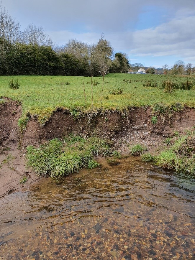
LiDAR offers itself as a good means to quantify large areas and allows a movement away from traditional erosion studies by using remote-sensing techniques to identify areas undergoing erosion. Studies such as Rose and Basher (2011) have used LiDAR successfully in catchments when combined with historical aerial photography to calculate riverbank erosion and meander migration on a five-decade basis. However, the usage of LiDAR to LiDAR comparisons is a more accurate means to determine erosion rates and can be widely replicated across various spatial scales or locations. This allows these areas to be targeted for management and allows the potential contributing areas and/or land uses waterway pollution inputs to be determined.
A study by Thoma et al., (2005) used LiDAR data to quantify and determine the contribution of sediment and nutrients in rivers such as P from riverbank erosion. LiDAR flights were used to create uniform 1 m digital elevation models of bare earth through vegetation stripping and interpolation. Image differencing was performed in GIS to determine the volume change over time. Mass wasting rates were calculated by multiplying net volume change with averages of bulk density. Inputs of sediment were then calculated by converting the mass-wasting rates into sediment load. Nutrient loads were derived by multiplying the mass of eroded sediment by the concentration of extractable P that was present in the samples. This allowed the contribution of riverbank erosion to total suspended sediment and nutrient loads in rivers to be determined. Such a methodology was adapted and used for the Blackwater catchment at the four study sites under question.
During August, several cores of riverbank material at each of the field sites were collected which represented typical riverbank strata for the field site under question. These underwent analysis for bulk density and total extractable Phosphorus. A freely available 2014 LiDAR 1 m DTM (digital terrain model) dataset on the OpenDataNI website covered the extent of the field sites in the Blackwater catchment giving a baseline date of imagery and riverbank position. The Centre for GIS and Geomatics within QUB flew drone flights across the field sites to produce a DSM (digital surface model) for July 2020. As this is a DSM, this contains vegetation returns and these must be removed to produce a DTM that represents bare earth elevation. Figure 2 shows the DSM for the Glenhoy site and the areas of vegetation and hedgerows are evident. Processing was performed in ArcPro to remove vegetation returns through the functions of imagery, pixel editor, and terrain filter to produce a DTM for each of the sites.
The two LiDAR datasets used for analysis covered a period of six years. Therefore, to calculate annual rates of erosion, sediment, and P loads, the volume change value calculated due to erosion was divided by six to give an average annual estimate of erosion. To calculate this average annual erosion rate, the sum of elevation differences between the two periods was divided by the spatial extent covered by each site’s buffered riverbank zones to give an average volume change per vertex (or rather each co-ordinate). The 2014 and 2020 LiDAR datasets were first clipped to the extent of the field sites under investigation before the function of raster calculator was used to produce an image differenced raster under the expression of; “2014 LiDAR Dataset – 2020 LiDAR dataset” as the difference in elevation values between the two scans. Under this particular expression, positive values represented areas of erosion, with negative values indicated areas of deposition. This was then clipped in size to the buffered riverbank zones of each site.
Whilst the study conducted by Thoma et al., (2005) was interested in net volume change of either erosion or deposition on a much larger scale, this work focused on the issue surrounding riverbank erosion and its potential to release sediment and nutrients. As such, using the function of extract by attributes with an expression of where “value > 0” any negative areas representing deposition were removed from the differencing rasters. These new rasters containing only positive values of erosion were used in the tool of zonal statistics to calculate the summed total of elevation differences at each vertex for each riverbank. This summed value was then divided by the spatial extent covered by the riverbank to give an average change in elevation per-vertex, which represents the average rate of erosion for the area under analysis.
To give an average annual erosion rate per year this value was divided by six. To calculate an average mass wasting rate this per annum average erosion rate was multiplied by the average bulk density. To calculate the average annual input of sediment to waterways for the entire riverbank this average mass wasting rate was multiplied by the spatial extent of the riverbank zones. Finally, to calculate the average annual inputs of total extractable phosphorus due to riverbank erosion, this average input of sediment was multiplied by the average total extractable phosphorus concentration to determine average phosphorus loading rates.
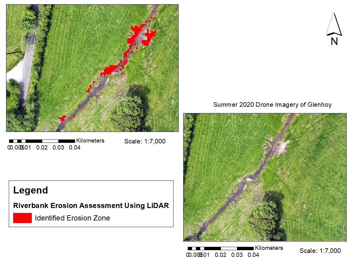
The following Table 1 shows the results for the Glenhoy site, which has issues surround direct livestock access into the waterway at this site causing riverbank destruction. This increases sediment release and there is an increased risk of nutrient enrichment through direct animal excretion into the waterway here. Figure 3 shows the identified zones of erosion using the LiDAR datasets that correlate closely to areas of bank destruction by livestock as shown in the summer 2020 drone imagery. These calculated results for each of the field sites help in understanding areas that are at the greatest risk of nutrient enrichment and can help to target and direct management intervention.
| Glenhoy | Average Annual Erosion Rate (cm yr-1) | Mass Wasting inputs of Sediment (kg yr-1) | Average Total Extractable Phosphorus Inputs due to Riverbank Erosion (mg yr-1) |
| Entire Site | 3.14 | 2.47 | 17.85 |
Table 1 showing the average annual riverbank erosion rates, mass wasting rates, and total extractable Phosphorus inputs calculated for the Glenhoy site
Whilst the calculations obtained for the Blackwater sites are average annual rates and inputs, considerations must be made upon the variable and dynamic nature of fluvial systems in terms of alternations of discharge and flow regimes concerning meteorological changes and how this may influence the rate of erosion. Under changing climatological conditions, this is an important factor for consideration, and this particular assessment technique of using LiDAR to quantify annual rates of erosion may be an interesting and novel methodology to monitor any changes in erosion rates under a changing climate.
In terms of future project work, the zones of erosion identified through the function of extract by attributes will be incorporated into a wider GIS model. This model aims to assess areas at-risk of nutrient and sediment enrichment in combination with datasets such as slope, soil nutrient hotspots, proximity to a waterway, etc to determine areas requiring management intervention to help achieve the EU WFD. Proposed fieldwork for the coming Winter months will also begin to look at establishing runoff plots to monitor sediment and nutrient losses with runoff alongside the continuation of water sampling at the study sites.
References
Thoma, D. P., Gupta, S. C., Bauer, M. E. and Kirchoff, C. E. (2005). Airborne laser scanning for riverbank erosion assessment. Remote Sensing of Environment, 95, 4, 493-501.
Rose, R. C. D. and Basher, L. R. (2011). Measurement of river bank and cliff erosion from sequential LIDAR and historical aerial photography. Geomorphology, 126, 1-2, pp. 132-147.
Sharpley, A. N., Daniel, T., Simms, T., Lemunyon, J., Stevens, R. and Parry, R. (2003). Agricultural Phosphorus and Eutrophication (2nd Edition). U.S. Department of Agriculture, Agricultural Research Service, ARS series 149.